Dancing With Qubits, First Edition: What’s in the book

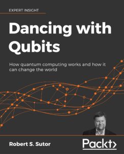
Cover of the book Dancing with Qubits

This morning I awoke to a very nice email from Tom Jacob, the Project Editor for my book at Packt Publishing. He said, in part,

We were able to successfully ship the book to our printers. …
Congratulations on achieving this milestone!

As I’ve mentioned before, my book was prepared using LaTeX and not Microsoft Word. I gave the publishers what was essentially the “camera-ready” PDF file from which to print. Hence the part about being able to “successfully ship” the book. In fact, I sent them the final PDF last night. I thought I was done on Friday, but yesterday I noticed an out-of-place citation in the section on the Bloch sphere and did a quick fix.

Now that the book is in production and there is absolutely nothing else I can do to fiddle with it, I’m going to show you the table of contents. I tried to have fun with some of the chapter and section titles. Once the book is published, I’ll be happy to discuss why I included this content or that.


Dancing with Qubits
How quantum computing works and
how it can change the world

Preface ix

1  Why Quantum Computing? 1

1.1 The mysterious quantum bit 2

1.2 I’m awake! 4

1.3 Why quantum computing is different 7

1.4 Applications to artificial intelligence 9

1.5 Applications to financial services 15

1.6 What about cryptography? 18

1.7 Summary 21

I  Foundations 23

2  They’re Not Old, They’re Classics 25

2.1 What’s inside a computer? 26

2.2 The power of two 32

2.3 True or false? 33

2.4 Logic circuits 36

2.5 Addition, logically 39

2.6 Algorithmically speaking 42

2.7 Growth, exponential and otherwise 42

2.8 How hard can that be? 44

2.9 Summary 55

3  More Numbers than You Can Imagine 57

3.1 Natural numbers 58

3.2 Whole numbers 60

3.3 Integers 62

3.4 Rational numbers 66

3.5 Real numbers 73

3.6 Structure 88

3.7 Modular arithmetic 94

3.8 Doubling down 96

3.9 Complex numbers, algebraically 97

3.10 Summary 103

4  Planes and Circles and Spheres, Oh My 107

4.1 Functions 108

4.2 The real plane 111

4.3 Trigonometry 122

4.4 From Cartesian to polar coordinates 129

4.5 The complex “plane†129

4.6 Real three dimensions 133

4.7 Summary 134

5  Dimensions 137

5.1 R2 and C1 139

5.2 Vector spaces 144

5.3 Linear maps 146

5.4 Matrices 154

5.5 Matrix algebra 166

5.6 Cartesian products 176

5.7 Length and preserving it 177

5.8 Change of basis 189

5.9 Eigenvectors and eigenvalues 192

5.10 Direct sums 198

5.11 Homomorphisms 200

5.12 Summary 204

6  What Do You Mean “Probably� 205

6.1 Being discrete 206

6.2 More formally 208

6.3 Wrong again? 209

6.4 Probability and error detection 210

6.5 Randomness 212

6.6 Expectation 215

6.7 Markov and Chebyshev go to the casino 217

6.8 Summary 221

II  Quantum Computing 223

7  One Qubit 225

7.1 Introducing quantum bits 226

7.2 Bras and kets 229

7.3 The complex math and physics of a single qubit 234

7.4 A non-linear projection 241

7.5 The Bloch sphere 248

7.6 Professor Hadamard, meet Professor Pauli 253

7.7 Gates and unitary matrices 265

7.8 Summary 266

8  Two Qubits, Three 269

8.1 Tensor products 270

8.2 Entanglement 275

8.3 Multi-qubit gates 283

8.4 Summary 295

9  Wiring Up the Circuits 297

9.1 So many gates 298

9.2 From gates to circuits 299

9.3 Building blocks and universality 305

9.4 Arithmetic 315

9.5 Welcome to Delphi 322

9.6 Amplitude amplification 324

9.7 Searching 330

9.8 The Deutsch-Jozsa algorithm 338

9.9 Simon’s algorithm 346

9.10 Summary 354

10  From Circuits to Algorithms 357

10.1 Quantum Fourier Transform 358

10.2 Factoring 369

10.3 How hard can that be, again 379

10.4 Phase estimation 382

10.5 Order and period finding 388

10.6 Shor’s algorithm 396

10.7 Summary 397

11  Getting Physical 401

11.1 That’s not logical 402

11.2 What does it take to be a qubit? 403

11.3 Light and photons 406

11.4 Decoherence 415

11.5 Error correction 423

11.6 Quantum Volume 429

11.7 The software stack and access 432

11.8 Simulation 434

11.9 The cat 439

11.10 Summary 441

12  Questions about the Future 445

12.1 Ecosystem and community 446

12.2 Applications and strategy 447

12.3 Access 448

12.4 Software 449

12.5 Hardware 450

12.6 Education 451

12.7 Resources 452

12.8 Summary 453

Afterword 455

Appendices 458

A  Quick Reference 459

A.1 Common kets 459

A.2 Quantum gates and operations 460

B  Symbols 463

B.1 Greek letters 463

B.2 Mathematical notation and operations 464

C  Notices 467

C.1 Creative Commons Attribution 3.0 Unported (CC BY 3.0) 467

C.2 Creative Commons Attribution-NoDerivs 2.0 Generic (CC BY-ND 2.0) 468

C.3 Creative Commons Attribution-ShareAlike 3.0 Unported (CC BY-SA 3.0) 468

C.4 Los Alamos National Laboratory 469

C.5 Trademarks 469

D  Production Notes 471

Other Books You May Enjoy 473

Index 477


Changes, clarifications, and errata


Previous: Drawing quantum circuits
Next: What about the eBook?

In December, 2019, Packt Publishing published my book Dancing with Qubits: How quantum computing works and how it can change the world. Through a series of blog entries, I talk about the writing and publishing process, and then about the content.

Dancing With Qubits, First Edition: Drawing quantum circuits

This entry is for people who use the LaTeX document preparation system, as I did in the book. It’s not a tutorial on LaTeX in general, but shows some techniques for drawing quantum circuits. To be direct, it’s pretty geeky for LaTeX people.

An early decision I had to make was how to draw quantum circuit diagrams in the book. Here’s an example of one:

A quantum circuit

This includes three Hadamard H gates, two S gates, a T gate, and a swap gate. Would I need to write my own drawing routines?

I really didn’t want to do that because of my time constraints but I also hoped that I could find something better. It didn’t take me long to do so: Alastair Kay’s excellent quantikx package on the CTAN Comprehensive TeX Archive Network. The documentation there is very good, but in this blog entry I’m going to show you how to evolve a simple circuit to have stylistic customizations that you might want to modify and use.

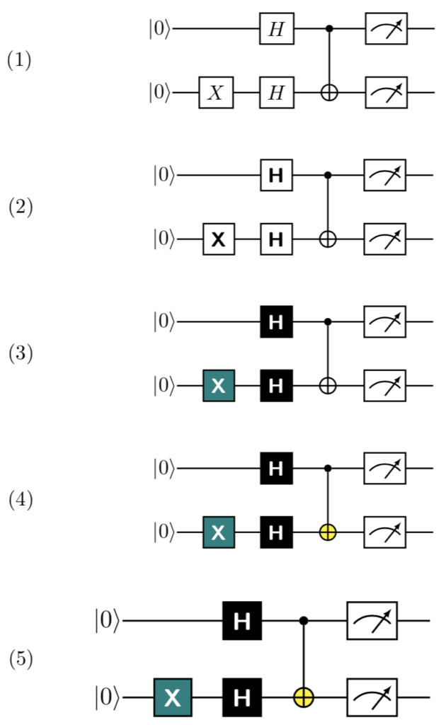
Below are five displayed versions of the same circuit. They are numbered on the left side.Five example circuits

The first is the default formatting from quantikz. It is perfectly fine and you can see similarly formatted circuits in research articles about quantum computing.

\begin{center}
    \begin{tikzpicture}
        \node[scale=1.0] {
            \begin{quantikz}
                \ket{0} & \qw       & \gate{H} & \ctrl{1}   & \meter{} & \qw \\
                \ket{0} & \gate{X}  & \gate{H} & \targ{}    & \meter{} & \qw
            \end{quantikz}
        };
    \end{tikzpicture}
\end{center}

The markup \ket{0} produces the |0> at the beginning of each wire, which is a horizontal line. \qw creates a segment of a quantum wire. \gate is the basic command for drawing a labeled gate with a rectangle. \meter is the quantum measurement operator. \ctrl{1} and \targ{} are the two parts of a CNOT two-qubit gate. \ctrl{1} is on the wire for the control qubit and extends a line down one wire. There the line meets the \targ{} (target) qubit and is drawn as a circle around a “+” sign.

In the second example, I’ve changed the font in the H and X gates.

\newcommand*{\gateStyle}[1]{{\textsf{\bfseries #1}}}
\newcommand*{\hGate}{\gateStyle{H}}
\newcommand*{\xGate}{\gateStyle{X}}

\begin{center}
    \begin{tikzpicture}
        \node[scale=1.0] {
            \begin{quantikz}
                \ket{0} & \qw            & \gate{\hGate} & \ctrl{1}   & \meter{} & \qw \\
                \ket{0} & \gate{\xGate}  & \gate{\hGate} & \targ{}    & \meter{} & \qw
            \end{quantikz}
        };
    \end{tikzpicture}
\end{center}

I added three LaTeX macros to encapsulate the new function and make it easier to reuse.

  1. \gatestyle puts its text in a bold sans serif font.
  2. \hGate draws the Hadamard H using \gatestyle.
  3. \xGate draws the X using \gatestyle.

While it is now easier to use \hGate and \xGate for text, it’s still wordy to use them as gates in a circuit. The third example defines two more macros, \circuitH and \circuitX, and shows how to set the background and font colors. For a printed book, you might want to have gates with backgrounds in different shades of gray. Alternatively, you could use the same background color for all the Clifford gates.

\newcommand*{\circuitH}{\gate[style={fill=black},label style=white]{\textnormal{\hGate{}}}}
\newcommand*{\circuitX}{\gate[style={fill=teal},label style=white]{\textnormal{\xGate}}}

\begin{center}
    \begin{tikzpicture}
        \node[scale=1.0] {
            \begin{quantikz}
                \ket{0} & \qw            & \circuitH & \ctrl{1}   & \meter{} & \qw \\
                \ket{0} & \circuitX      & \circuitH & \targ{}    & \meter{} & \qw
            \end{quantikz}
        };
    \end{tikzpicture}
\end{center}

Now let’s set the color for the circle in \targ.

\newcommand*{\circuitTarget}[1]{\targ[style={fill=yellow}]{#1}}

\begin{center}
    \begin{tikzpicture}
        \node[scale=1.0] {
            \begin{quantikz}
                \ket{0} & \qw            & \circuitH & \ctrl{1}         & \meter{} & \qw \\
                \ket{0} & \circuitX      & \circuitH & \circuitTarget{} & \meter{} & \qw
            \end{quantikz}
        };
    \end{tikzpicture}
\end{center}

I think you get the idea. You can also set the background color for \meter, which I leave to you as an exercise. Note that in the April, 2019, version of quantikx, you could not change the color of the line inside the \meter graphic. You need to copy and redefine the macro (or create a new macro) to do that.

Finally, let me explain what that [scale=1.0] is doing after the \node. This allows you to scale the entire drawing and make it larger or smaller. However, it does not change the text size. The fifth example shows the fourth example drawn 20% larger.

\begin{center}
    \begin{tikzpicture}
        \node[scale=1.2] {
            \begin{quantikz}
                \ket{0} & \qw            & \circuitH & \ctrl{1}         & \meter{} & \qw \\
                \ket{0} & \circuitX      & \circuitH & \circuitTarget{} & \meter{} & \qw
            \end{quantikz}
        };
    \end{tikzpicture}
\end{center}

Here is the complete LaTeX file I used to generate the examples:


\usetikzlibrary{quantikz}

\mainmatter


\begin{center}
    \begin{tikzpicture}
        \node at (-5,0) {(1)};
        \node[scale=1.0] {
            \begin{quantikz}
                \ket{0} & \qw       & \gate{H} & \ctrl{1}   & \meter{} & \qw \\
                \ket{0} & \gate{X}  & \gate{H} & \targ{}    & \meter{} & \qw
            \end{quantikz}
        };
    \end{tikzpicture}
\end{center}


\newcommand*{\gateStyle}[1]{{\textsf{\bfseries #1}}}
\newcommand*{\hGate}{\gateStyle{H}}
\newcommand*{\xGate}{\gateStyle{X}}

\begin{center}
    \begin{tikzpicture}
        \node at (-5,0) {(2)};
        \node[scale=1.0] {
            \begin{quantikz}
                \ket{0} & \qw            & \gate{\hGate} & \ctrl{1}   & \meter{} & \qw \\
                \ket{0} & \gate{\xGate}  & \gate{\hGate} & \targ{}    & \meter{} & \qw
            \end{quantikz}
        };
    \end{tikzpicture}
\end{center}


\newcommand*{\circuitH}{\gate[style={fill=black},label style=white]{\textnormal{\hGate{}}}}
\newcommand*{\circuitX}{\gate[style={fill=teal},label style=white]{\textnormal{\xGate}}}

\begin{center}
    \begin{tikzpicture}
        \node at (-5,0) {(3)};
        \node[scale=1.0] {
            \begin{quantikz}
                \ket{0} & \qw            & \circuitH & \ctrl{1}   & \meter{} & \qw \\
                \ket{0} & \circuitX      & \circuitH & \targ{}    & \meter{} & \qw
            \end{quantikz}
        };
    \end{tikzpicture}
\end{center}


\newcommand*{\circuitTarget}[1]{\targ[style={fill=yellow}]{#1}}

\begin{center}
    \begin{tikzpicture}
        \node at (-5,0) {(4)};
        \node[scale=1.0] {
            \begin{quantikz}
                \ket{0} & \qw            & \circuitH & \ctrl{1}         & \meter{} & \qw \\
                \ket{0} & \circuitX      & \circuitH & \circuitTarget{} & \meter{} & \qw
            \end{quantikz}
        };
    \end{tikzpicture}
\end{center}


\begin{center}
    \begin{tikzpicture}
        \node at (-4.4,0) {(5)};
        \node[scale=1.2] {
            \begin{quantikz}
                \ket{0} & \qw            & \circuitH & \ctrl{1}         & \meter{} & \qw \\
                \ket{0} & \circuitX      & \circuitH & \circuitTarget{} & \meter{} & \qw
            \end{quantikz}
        };
    \end{tikzpicture}
\end{center}


Previous: My five rules for making revisions from editorial comments
Next: What’s in the book

In December, 2019, Packt Publishing published my book Dancing with Qubits: How quantum computing works and how it can change the world. Through a series of blog entries, I talk about the writing and publishing process, and then about the content.

Dancing With Qubits, First Edition: My five rules for making revisions from editorial comments

Cover of the book Dancing with QubitsToday I finished making revisions to the book based on comments from the proofreader. All told, there have been five people providing feedback and comments for how I should modify, fix, and improve the content:

  • me
  • the technical reviewer
  • the project editor
  • the development editor
  • the proof reader

My editing started as soon as I started writing, but it has been an iterative process. The technical reviewer made sure what I said was correct, and occasionally caught typos. The project editor, Tom Jacob, focused on the workflow of the overall process and contributed comments about the physical structure of the book and what publisher content should be included.

The development editor, Dr. Ian Hough, has been my constant online companion for the last few months. It is his responsibility to sign off on the final content. He provided suggestions and ideas, and checked that I made good revisions. Sometimes he corrected the revised text when I made mistakes (hey, it was late!). The proofreader did the nitty-gritty editing for punctuation and clarity. Ian filtered those suggestions and passed them along to me. He then checked, again, that I had done the correct revisions.

LaTeX markup showing change bars

Some “suggestions” were really just that. They were optional, but I incorporated almost all of them.

Here are five things I’ve kept in mind or learned through this editing and revision process:

  1. This is not about my ego, it’s about producing the best content.
  2. The mathematics and science must be correct. (I knew this!)
  3. If anyone thinks something is unclear, then I rewrite it.
  4. I need to use many more commas.
  5. It’s important to correctly use the right word in standard pairs such as “that/which” and “already/all ready.”

My bonus rule is to eliminate superfluous words.


Previous: The writing process – what format?
Next: Drawing quantum circuits

In December, 2019, Packt Publishing published my book Dancing with Qubits: How quantum computing works and how it can change the world. Through a series of blog entries, I talk about the writing and publishing process, and then about the content.

Dancing With Qubits, First Edition: The writing process – what format?

Cover of the book Dancing with QubitsBefore I discuss what and I how I wrote, let me talk about the markup of the book. By “markup” I mean the underlying format of the content that determines its structure such as the title page, table of contents, parts, chapters, sections, paragraphs, bibliography, and the index, along with font styles and sizes.

In my experience, most publishers, both traditional and online, prefer you to use Microsoft Word to create the book, and it has its own underlying markup language that you typically never see. In a more-or-less what-you-see-is-what-you-get way, you can write and style the book.The publishing workflow is often based on this choice.

My requirements for the book creation process included:

  • beautiful math rendering, both in sentences and displayed multi-part formulas,
  • built-in support for generating diagrams,
  • easy methods to change formatting throughout the book quickly, and
  • good support for working quickly on a large text.

Regarding the size of the book, in early 2019 I thought the book would come in around 300 pages and I would have a complete draft on September 1. I ended up writing a book with slightly more than 500 pages with the first full draft delivered on October 9. I had full drafts of various chapters before then, but that was the first time there were no sections with TODO markers.

ebook on iPadWord has come a long way on many of these requirements, especially the math, though it can be very laborious to create a book with hundreds or thousands of formulas. Here’s the real problem though: eBooks with math in them often look terrible if you put them in a reflowable format. That is, if you let, say, your Amazon Kindle change the fonts and the line widths, the math just doesn’t look right.

People argue about this forever, but there is an excellent chance that you will end up with fuzzy, misaligned expressions that are the wrong size compared to the surrounding text. So, I early on made the decision that the eBook would not be reflowable. Since that was the case, there was no reason for me to stick with Word. I decided to markup the book in LaTeX. Luckily, Andrew Waldron at Packt Publishing agreed. [Though see this later development regarding the eBook.]

With LaTeX, you have complete and arbitrary control over all parts of the formatting. There are thousands of packages that make your life easier by providing significant functionality that you would not want to write yourself.

LaTeX has

  • the best math formatting facilities of any system,
  • packages like pgf/tikz for creating diagrams,
  • a full macro programming language for formatting control and calculations, and
  • easy ways to break a document into sections so you can work on one part at a time.

If you get into macro programming, things can get complicated. I’ve been doing it for 30 years, so it doesn’t faze me. Here are two good books on LaTeX to get you started:


Previous: Last minute tweaks to my quantum computing book cover
Next: My five rules for making revisions from editorial comments

In December, 2019, Packt Publishing published my book Dancing with Qubits: How quantum computing works and how it can change the world. Through a series of blog entries, I talk about the writing and publishing process, and then about the content.

Dancing With Qubits, First Edition: Last minute tweaks to my quantum computing book cover

With a month to go before publication, we are still making last minute tweaks to my quantum computing book Dancing with Qubits. We made two changes to the cover this week. Can you spot the differences?

The old version is the first image, the new version is the second:
old book cover Cover of the book Dancing with Qubits
How do you interpret the change made in the subtitle?


Previous: Let me preface my remarks with …
Next: The writing process – what format?

In December, 2019, Packt Publishing published my book Dancing with Qubits: How quantum computing works and how it can change the world. Through a series of blog entries, I talk about the writing and publishing process, and then about the content.

Dancing With Qubits, First Edition: Let me preface my remarks with …

Cover of the book Dancing with QubitsWay back in 1992, Springer-Verlag published my first book Axiom: The Scientific Computation System, co-authored with the late Richard D. Jenks. Since then I’ve thought of writing other books, but work and life in general caused enough inertia that I never got around to it.

I first got involved with IBM’s quantum computing effort in early 2016. By 2018, I was again thinking of writing a book and this subject was an obvious candidate. How would I start? What would I say? What was my perspective on the topic given that there were already some excellent books?

To write a book, you have to start writing. This is obvious, but no less true and important. In the summer of 2018, I started writing what I thought would be the introduction to the book. My perspective was, and is, very much from the mathematical and computer science directions. To be clear, I am not a physicist. If I could produce a coherent introduction to what I thought the book would cover, I might convince myself that it would be worth the hundreds of hours it would take to complete the project.

When I recently announced that the book was available for pre-order, my industry colleague Jason Bloomberg asked:

“So where does it fall on the spectrum between ‘totally accurate yet completely impenetrable’ and ‘approachable by normal humans but a complete whitewash’?”

I responded:

“I bring you along … to give you the underlying science of quantum computing so you can then read the “totally accurate but formally impenetrable” texts.”

I decided that I would cover the basic math necessary to understand quantum computing, and then get into quantum bits (qubits), gates, circuits, and algorithms. Although readers with the necessary background (or perhaps a good memory of that background) can skip the mathematical fundamentals, I decided to take people through the algebra and geometry of complex numbers, linear algebra, and probability necessary to understand what qubits are and what you can do with them.

That early draft of the book’s introduction described roughly 15 chapters divided into three parts. The final book has 12 chapters and 2 parts. That introduction eventually became the Preface. Part III eventually became Chapter 1.

It’s much tighter than what I imagined it would be, but there is still material I could have covered. There’s a natural tendency to want to add more and more, but I kept asking myself “What is this book about? How deeply do I want to go? Am I getting off track? Will I ever finish?”.

As 2018 went on, I kept tweaking the introduction and I started talking to publishers. In November, I started writing what was then the first chapter. Although I started in Microsoft Word, which is overwhelmingly the format of choice for many publishers, I quickly switched to LaTeX. This produced a far more beautiful book, but also placed constraints on how I could publish the book.

With this as teaser, in future entries I’ll talk more about the writing process, choices I made, LaTeX packages I used and macros I wrote, deciding how to publish the book, and working with editors. Once the book is available, I’ll talk about the specific content and why I included what I did.


Next: Last minute tweaks to my quantum computing book cover

In December, 2019, Packt Publishing published my book Dancing with Qubits: How quantum computing works and how it can change the world. Through a series of blog entries, I talk about the writing and publishing process, and then about the content.

My Visual Studio Code extensions for LaTeX and Python

I’m in the final stages of writing a book about quantum computing using LaTeX and I also do a lot of Python programming when I get a chance. A couple of years ago, I decided to try using the Visual Studio Code editor and I just love it. I’ve used dozens of programming editors in my life (vi, not emacs, thank you very much), and VSCode has the best functionality of all of them.

One of its best features is its extension architecture. Though I experiment with various extensions occasionally, I keep a core set. If I am going to so something special such as editing Markdown text, I will use an extra extension or two until I am done with the task and then uninstall them.

These are the extensions I use now for LaTeX editing and Python coding. They are all available in the editor through the Marketplace.

  • Blank Line Organizer – removes extraneous extra lines that creep into text while editing
  • Bookmarks – as you would suspect, allows you to set a bookmark somewhere in a file and then jump back to it quickly
  • Bracket Pair Colorizer 2 – paints matching parentheses, brackets, and curly brackets in the same color. I’ve tried the original and Rainbow Brackets, and none of these three are perfect. These version is the fastest and mostly best.
  • change-case – provides many options for changing the case (e.g., uppercase, lowercase, sentence case) of selected text
  • Code Runner – helps execute code in the environment
  • Code Spell Checker – tells you when a word has questionable spelling, though not good on suggesting alternatives. You can put comments in the file saying which words to ignore or store them in a file in the folder.
  • LaTeX Workshop – the workhorse large set of code to assist in editing LaTeX markup. I don’t use all the features and I still run things like pdflatex from the command line, but it is hugely helpful. As an aside, you probably want to get latexindent running on your machine if possible.
  • latex-count – simple add-on that shows how many non-markup words are in your document
  • MagicPython – syntax highlighter for Python
  • Python – the main set of code providing Python editing and execution
  • qiskit-vscode – editing and execution support for the open source Qiskit quantum computing development platform
  • Rewrap – rewraps lines of text. Useful when LaTeX content gets too ragged.
  • Settings Sync – saves your editor setting on GitHub so you can have the same environment across machines.

Recap: NanoDays with a Quantum Leap at the Museum of Science, Boston

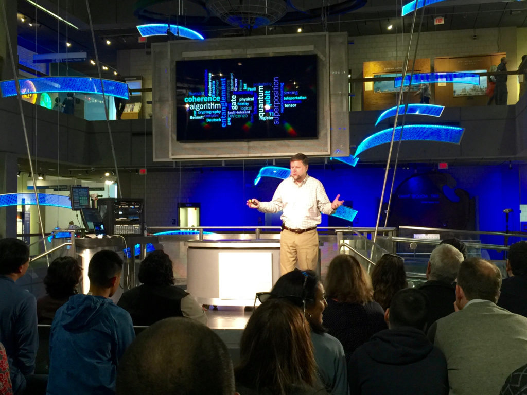
It was a beautiful spring day in Boston last Saturday, April 6, when my IBM Q colleague Melissa Turesky and I headed to the Museum of Science on the Charles River. It was a special event, “NanoDays with a Quantum Leap,” and I spoke about the IBM Q quantum computing program and how people could start coding it today.

I was most happy to see how many young people were at the museum and participating in the NanoDays events. A lot of what we are doing now with quantum computing is education and I hope that exhibits like this will encourage girls and boys to learn more about the area. I’d love to have someone tell me in 10 years that the museum exhibit inspired them to pursue a quantum-related STEM career.

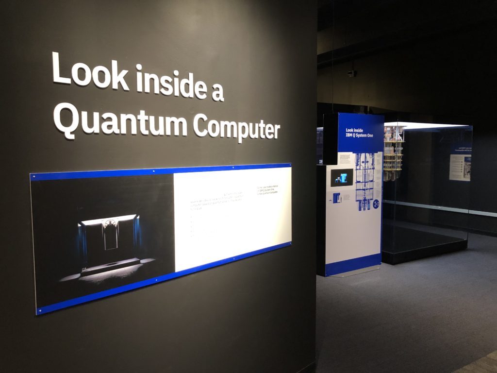
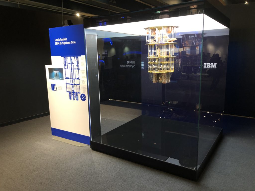
Since 2016, over 100,000 people have used the IBM Q Experience and they have run over 9.5M executions. A 50 qubit model of the IBM Q System One will be in residence as part of the quantum exhibit until the end of May.

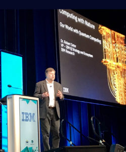
Bob Sutor speaking at the Museum of Science, Boston, on April 6, 2019. Photo by Carol Lynn Alpert.
IBM Q quantum computing exhibit at the Museum of Science. Boston, in April, 2019

My #BCTECHSummit 2019 talk

Bob Sutor speaking #BCTECHSummit in Vancouver in March, 2019
Photo courtesy of IBM Canada

I spoke this morning about quantum computing at #BCTECHSummit in Vancouver, British Columbia. Here are some of the points I emphasized:

  • The mainstream efforts including IBM Q are universal quantum computing systems with the eventual goal of full fault tolerance.
  • However, we believe “Quantum Advantage,” where we show significant improvement over classical methods and machines, may happen in the next decade, well before fault tolerance.
  • Don’t say “quantum computing will.” Say it “might.” Publish your results and your measurements.
  • Since May, 2016, IBM has hosted the IBM Q Experience, the most advanced and most widely used quantum cloud service. Over 100,000 users have executed close to 9 million quantum circuits. There is no charge for using the IBM Q Experience.
  • Qiskit is the most advanced open source framework for programming a quantum computer. It has components that provide high level user libraries, low level access, APIs for connecting to quantum computers and simulators, and new measurement tools for errors and performance.
  • Chemistry, AI, and cross-industry techniques such as Monte Carlo replacements are the areas that show great promise for the earliest Quantum Advantage examples.
  • The IBM Q Network is built around a worldwide collection of hubs, direct partnerships, academic memberships, and startups working accelerate educations and to find the earliest use cases that demonstrate Quantum Advantage.
  • Last week IBM Q published “Cramming More Power Into a Quantum Device” that discussed the whole-system Quantum Volume measurement, how we have doubled this every year since 2017, and how we believe there is headroom to continue at this pace.

Talk: The state of quantum computing in 2019

Here’s a video of the session that my IBM Q colleague Anthony J. Annunziata and I led at IBM Think in San Francisco a couple of weeks ago.

If I seem slightly breathless, I was. I had about 4 minutes to get from a client meeting in Moscone North to the speaking venue in Moscone South.

Click on the image to go to the video.

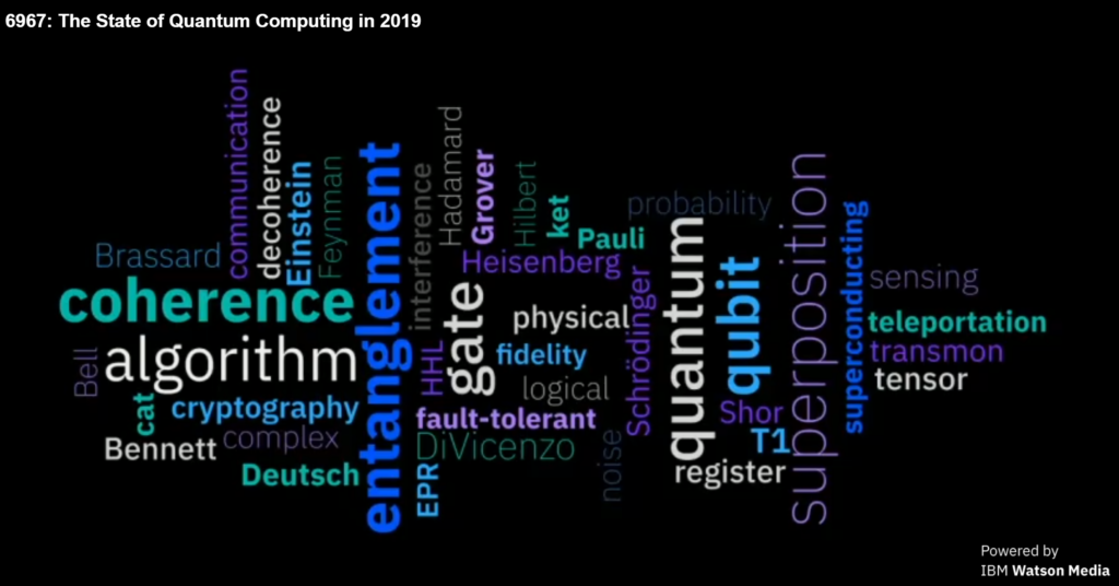
Slide from Think 2019

Math and Analytics at IBM Research: 50+ Years

Soon after I arrived back in IBM Research last July after 13 years away in the Software Group and Corporate, I was shown a 2003 edition of the IBM Journal of Research and Development that was dedicated to the Mathematical Sciences group at 40. From that, I and others assumed that this year, 2013, was the 50th anniversary of the department.

Herman Goldstine at IBM Research

I set about lining up volunteers to organize the anniversary events for the year and sent an email to our 300 worldwide members of what is now called the Business Analytics and Mathematical Sciences strategy area. Not long afterwards, I received a note from Alan Hoffman, a former director of the department, saying that he was pretty sure that the department had been around since 1958 or 59. So our 50th Anniversary became the 50+ Anniversary. Evidently mathematicians know the theory of arithmetic but don’t always practice it correctly

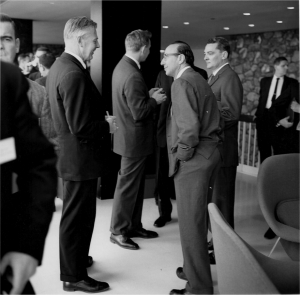
The first director of the department was Herman Goldstine who joined after working on the ENIAC computer and a stint at the Institute for Advanced Study in Princeton. Goldstine is pictured in the first photo on the right at a reception at the T.J. Watson Research Center in the early 1960s. Goldstine died in 2004, but all other directors of the department are still alive.

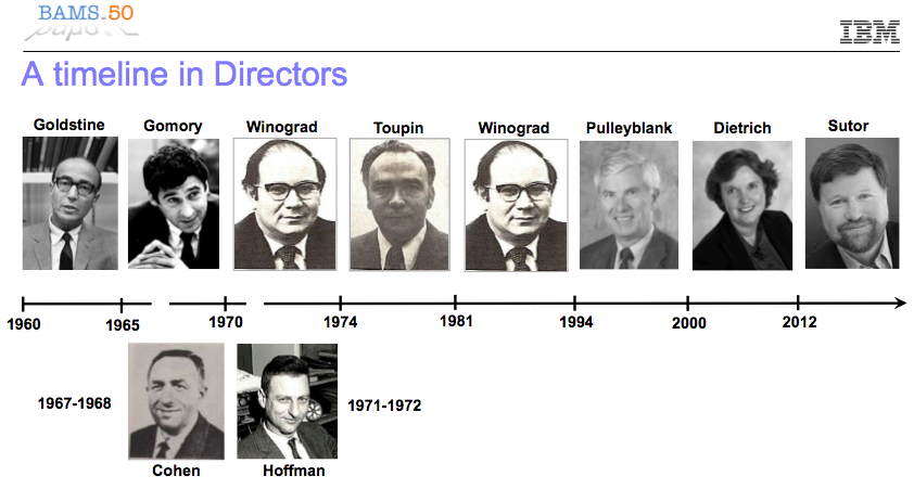
Directors of the Mathematical Sciences Department at IBM Research

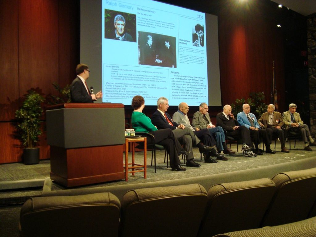
We decided that the first event of the year celebrating the (more than) half century of the department would be a reunion of the directors for a morning of panel discussions. This took place this last Wednesday, May 1, 2013.

Reunion of the directors of the Math Sciences Department at IBM Research
Photo credit: Mary Beth Miller

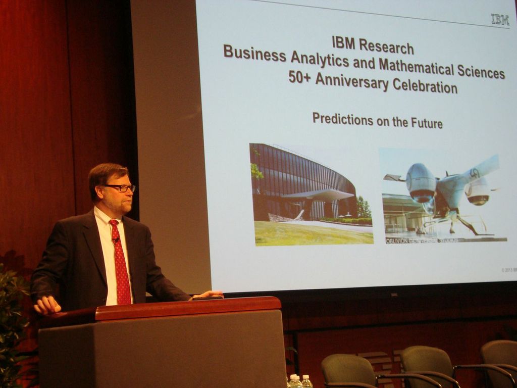
I started the day by giving a glimpse of what the department looks like today: the above-mentioned 300 Ph.D.s, software engineers, postdocs, and other staff distributed over the areas of optimization, analytics, visual analytics, and social business in 10 of IBM’s 12 global labs.

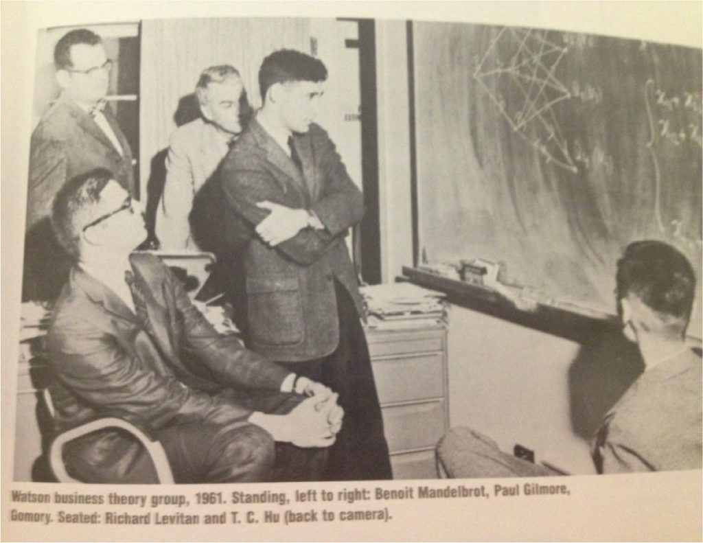
I then introduced our panel pictured in the photo above. From left to right we have me, Brenda Dietrich, Ralph Gomory, Benoit Mandelbrot, and other IBM researchers pondering a math problem

My goal for the discussion was to go back and look at some of the history and culture of the math department over the last five decades. I was hoping we would hear anecdotes and stories of what life was like, the challenges they faced, and the major successes and disappointments.

Other than a few questions I had prepared, I wasn’t sure where our conversation would go. The many researchers who joined us in the auditorium at the T. J. Watson Research Center in Yorktown Heights, NY, or via the video feed going out to the other worldwide labs would have a chance to ask questions near the end of the morning.

I’m not going to go over every question and answer but rather give you the gist of what we spoke about.

  • Ralph Gomory reminded us that the department was started in a much different time, during the Cold War. The problems they were trying to solve using the hardware and the software of the day were often related highly confidential. However, every era of the department has had its own focus, burning problems to be solved, and operational environment.
  • Hirsh Cohen got his inspiration for the mathematics he did by solving practical problems such as those related to the large mainframe-connected printers. Many people feel that mathematics shouldn’t stray too far from the concrete, but it is not that simple. This isn’t just applied mathematics, it is a way of looking for inspiration that may express itself in more theoretical ways. The panelists mentioned more than once that the original posers of business or engineering problems might not recognize the mathematics that was developed in response. (I think there is nothing wrong with theoretical mathematics with no direct connection to the physical world, but there are some areas of mathematical pursuit that I think are just silly and of marginal pure or applied interest.)
  • In response to my question about balancing business needs with the desire to advance basic science, Shmuel Winograd told me I had asked the wrong question: it was about the integration of business with basic science, not a partitioning of time or resources between them. This very much sets the tone of how you manage such a science organization in a commercial company. The successful integration of these concerns may also be why IBM Research is pretty much the sole survivor of the industrial research labs from the 1950s and 1960s.
  • There was general consensus that it is difficult to get a researcher to do science in an area that he or she fundamentally does not want to work. This was redirected to the audience members who were reminded to understand what they loved to do and then find a way to do it. (This sounded like a bit of a management challenge to me, and I suspect I’ll hear about it again.)
  • Time gives a great perspective on the quality and significance of scientific work that is just not obvious while you are the middle of it. This is one of the reasons why retrospectives such as this can be so satisfying.
Discussing the future of BAMS
Photo credit: Mary Beth Miller

After the first panel and coffee break, we came back and I started the session looking at the future of the department instead of the history. We have an internal department social network community in IBM Connections and I started by summarizing some of the suggestions people came up with about what we’ll be doing in the department in five, ten, and twenty years.

Sustainability, robotic applications of cognitive computing, and mathematical algorithms for quantum computing were all suggested. Note that his was all fun speculation, not strategy development!

Eleni Pratsini, Director of Optimization Research, and Chid Apte, Director of Analytics Research, then each discussed technical topics that could be future areas for scientific research as well as having significant business use.

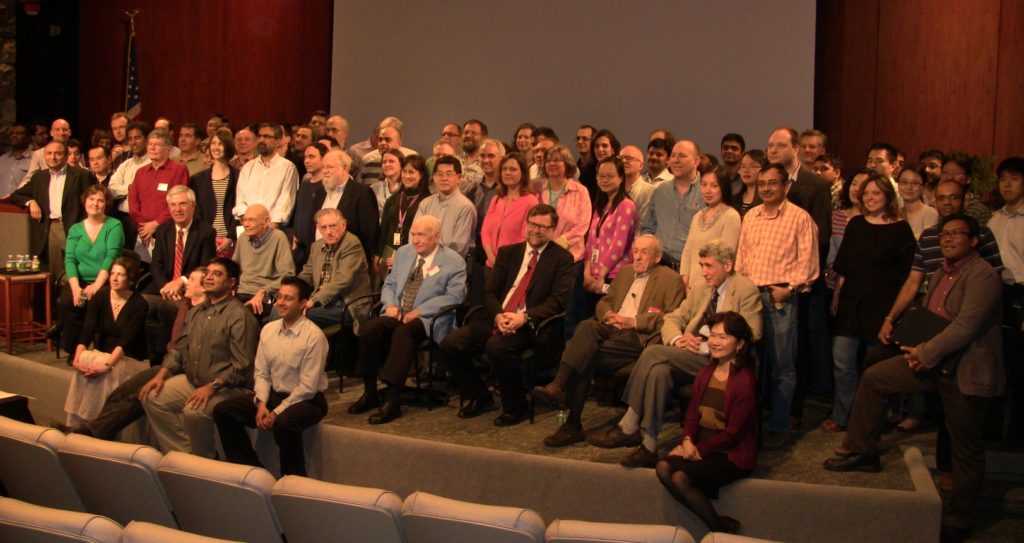
After the final Q&A session, we got everyone on stage for a group photo.

Photo credit: Steve Hamm

One thing that struck me when we were doing the research through the archives was how much more of a record we have of the first decade of the department than we do of the 40+ years afterwards. In those early days, each department did a typed report of its activities which was then sent to management and archived.

With the increasing use of email and, much later, digital photos, we just don’t have easy if any access to what happened month by month. As part of this 50+ Anniversary, I’m going to organize an effort to do a better job of finding and cataloging the documents, photos, and video of the department.

This should make it easier for future celebrations of the department’s history. I suspect I’m not going to make it to the 100th anniversary, but I just might get to the 75th. For the record for those who come after me, that will be in 2034.

Verified by MonsterInsights